Adding counter tables on XISA™

Getting accountable

Welcome back network enthusiasts! We're Xsight-ed to continue our deep dive into the inner workings of programmable network switches using the X-Switch Instruction Set Architecture (XISA).

Our journey began with the fundamentals – exploring a basic cross-connect example to understand how packet forwarding works at the microcode (uCode) level. We then took a significant step forward by tackling a Simple IPv4 switching program, which introduced concepts such as packet parsing to identify headers and fields, preloading data into MAP registers, and performing Longest Prefix Match (LPM) lookups incorporating VRF functionality.

Later, we added IPv4 header validation code and learned to modify the TTL and update the header checksum. Our code became more robust, detecting and subsequently dropping many kinds of packets, thereby preventing them from leaking into the network or being mis-forwarded.

Now, let's place ourselves in the shoes of a system administrator. If all they have to go on are the standard SNMP MAC counters, then any discrepancy between the total number of packets sent or received would indicate a problem — but wouldn't reveal its nature. Ideally, we would want to make sure that packets didn't just vanish without leaving a trace. The best way to achieve such visibility is by counting the packets — especially the ones that were dropped (for example, because of a failed validity check, like the one we introduced in our previous article).

This is precisely the functionality we want to add. In today's example we'll walk you through how to add a counter table to a program written using XISA. We'll go step-by-step — starting with the necessary definitions and code updates — and also discuss a number of different ways to organize and use counters efficiently.

To begin with, let's define the functionality that we want to add to our program.

We want to add several counters per ingress port to track the following:

In addition to counting the number of packets we will also show how to count the number of bytes in them – useful when billing the customers for their internet traffic.

The basic plan

Overall, this example's program structure will be the same as in the previous example; here we'll concentrate mostly on adding the counters.

First, let us schematically show how we'd like to have our counters organized.

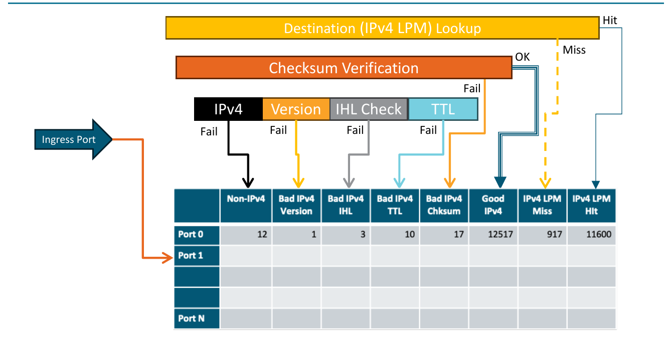
Figure 1. Conceptual counter organization^[1]

It seems natural to organize the counters in a sort of two-dimensional array (matrix) with the rows corresponding to the port numbers and the columns corresponding to the various events (causes) that can be enumerated.

Here is one way to enumerate the packet types:

Table 1. Packet type enumeration

To implement the counters, we'll also need several primitives with the ability to:

• Store counter values so that they can persist between packets.
• Increment the stored values.
• Determine the packet length in bytes (once we decide to add this capability).

XISA architecture provides specialized counter tables that offer both the persistent counter storage and the ability to increment counters atomically^[2], a very important feature given the highly parallel nature of packet processing in XISA.

XISA Counter tables can be thought of as arrays of counter entries, accessible via a counter index, with the number of entries (aka rows) controlled by programmer. The entry format is also flexible: each entry can contain either a single value, or a pair of values and those values can be either 32 or 64-bit wide. Besides that, no special semantics are assigned. For example, it's up to the programmer to decide which value in a pair will contain the packet counter and which one will contain a byte counter. In fact, one can think of them not as specialized counter objects, but as generic registers that support store, add, subtract and even retrieve operations^[3].

Based on the description above, we can easily imagine XISA counter tables as one-dimensional arrays, as depicted in Figure 2 below:

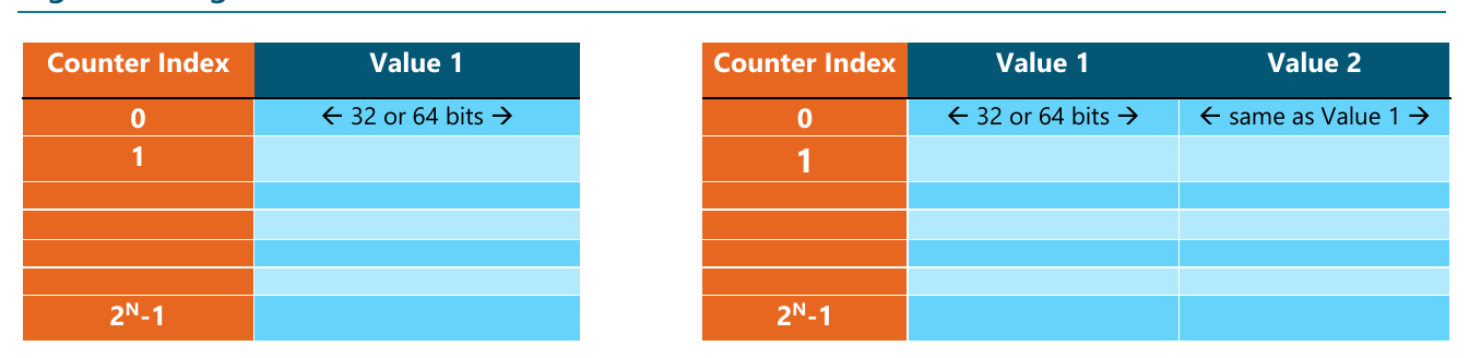
Figure 2. Single and double counters

There are two options we can use to implement a two-dimensional array, as depicted in Figure 1. We could create multiple counter arrays (one per column), but that option may be a bit heavy and does not scale well. A better way would be to linearize the two-dimensional array, converting it into a single-dimensional one by first placing the cells from the first row, then placing the cells from the next row, etc.

In this case, the index I, corresponding to the cell (the element) from row R and column C, can be calculated using a very simple formula I = R × N + C, where N is the number of elements in the row (i.e., the number of different counters we want to collect). This is a classic technique that is used to implement multi-dimensional arrays in traditional programming languages, such as C.

As a result, our algorithm will begin to look like this:

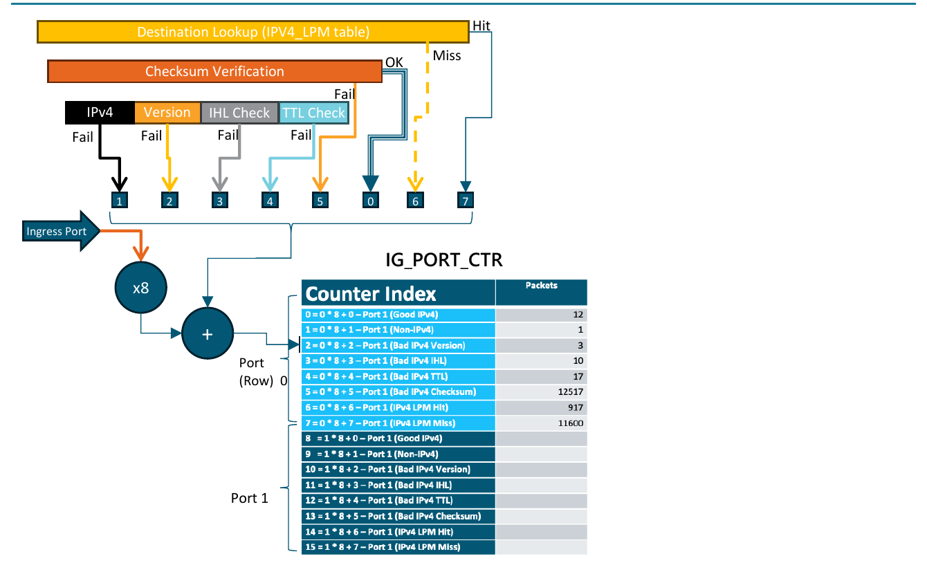
Figure 3. Collecting counters in a linearized counter array

A careful reader might have noticed by now that the counter table (let's call it Ingress Port Counter Table or IG_PORT_CTR for short) might be updated more than once per packet.

Indeed, if the packet is a valid one, the algorithm calls for updating the PACKET_TYPE_GOOD_IPV4 counter for the ingress port. Then, after completing the IPV4_LPM lookup, we'll need to update either the PACKET_TYPE_IPV4_LPM_HIT or PACKET_TYPE_IPV4_LPM_MISS counter for the same port based on the lookup outcome.

This might look like a problem to those used to working with pipeline-based programmable devices where it's very typical to allow accessing of any table, counter or similar resource, no more than once for a given packet^[4]. In those systems, we would need to use two separate counter tables: one to count good and bad IPv4 packets and another one to count the packets that hit or missed the IPv4_LPM table.

Fortunately, XISA allows multiple accesses to any object, such that we can easily place all the counters in a single table.

Now let's explore the required microcode updates.

Next, let's define the layout of the entries. As always, they consist of a key and data.

Since the port numbers in the X2 device are 8 bits wide, and since we defined 8 counter categories, the key can be 11-bits-wide. We can add its definition to the "struct" section of xdefs.json.

Figure 5. Defining the entry key format for the ingress port counter table

1{ "name": "IgPortCtrKey",2  "description": "Ingress Port Counter Entry Key (port * N + type)",3  "fields": [4    { "type": "BitField", "name": "ctr_index", "size": 11, "value": 0 }5  ]6},

We should also define the entry contents (the value), which is comprised of two 64-bit fields (counters), one for the packets and one for the bytes. The names of these fields can be arbitrary, but the order must match the program code:

Figure 6. Defining the entry value format for the ingress port counter table

1{ "name": "IgPortCtrValue",2  "description": "Ingress Port Counter Table Entry Value",3  "fields": [4    { "type": "BitField", "name": "packets", "size": 64, "value": 0 },5    { "type": "BitField", "name": "bytes",   "size": 64, "value": 0 }6  ]7}

After these preparations we can add the table definition to xdefs_table.json.

Figure 7. Defining the ingress port counter table

1{ "name": "IG_PORT_CTR",2  "description": "Ingress Port Counter Table. The index is computed using the formula port_number * PACKET_TYPE_MAX + packet_type",3  "id": "IG_PORT_CTR_TABLE_ID",4  "type": "Counters",5  "key_size": 11,6  "size": 2048,7  "ctr_type": "CTR_TYPE_DOUBLE",8  "ctr_size": "CTR_SIZE_8_BYTES",9  "key": "IgPortCtrKey",10  "value": "IgPortCtrValue"11}

• Line 1: Here we define the table name, "IG_PORT_CTR".
• Line 3: Here we specify the table ID, using the constant name that utilizes the definition, see Figure 4.
• Line 4: We need to specify the table type (Counters), as mentioned already, a specialized, predefined table type in XISA. This information is crucial for table provisioning and for allowing the special instructions to operate on this table.
• Lines 5: We need to specify the key width (in bits). It's very important to ensure that the key width matches the definition of the key that is referenced in Line 9 and defined in Figure 5.
• Line 6: Here we specify the number of entries, so that the table can be properly allocated.
• Line 7: Counter type indicates whether the table entry contains one or two counters. We chose entries that contain two counters each. This parameter must match the entry value definition, referenced on line 10 and defined in Figure 6.
• Line 8: Counter size specifies the size of the counters. If the counter table contains two counters, both will have the same width. The programmer can define either 4- or 8-byte-wide counters. This parameter must, however, match the entry value definition, referenced in line 10 and defined in Figure 6.
• Lines 9 and 10: Here we reference the structures that define the layout of the entry key and value. The layouts themselves have been defined in Figure 5 and Figure 6, correspondingly.

That's it! We've added a new table to our data plane program, and it can now be used in the microcode as well as accessed by the control plane APIs.

Computing the counter base index

Before we can increment a counter corresponding to the given ingress port, we need to compute the base counter index. As discussed above and depicted in Figure 3, we need to multiply the ingress port number by the number of different counters we are collecting.

In our case, this is easy. Since the total number of counters we want to collect per port is equal to 8 – we can simply shift the port number by three bits and get the desired number.

The ingress port number is always available to the MAP programs in bits 7:0 of the standard metadata (SMD) that is automatically passed with each packet in register R7.0 as depicted in Figure 8.

Figure 8. XISA standard metadata (SMD)

Thus, we can easily shift that value using the SHLI (SHift Left Immediate) instruction, available to us in the XISA, and store it for future use, e.g. in a register R1.2 as depicted below:

Figure 9. Computing the ingress port counter index by shifting the ingress port number

1S1    SHLI.CD    R1.2, R7.0, 0, 8, 3

However, what should we do if the number of counters is not a power of two?

In following the XISA documentation, you'll quickly realize that XISA does not offer a multiply instruction^[5]. We can, of course simulate multiplication through a series of shifts, adds and subtracts, but that will require us to change this multiplication code every time we need to change the number of counters we collect.

Fortunately, there is a better way – we can precompute those values in the control plane! Remember that every time a packet is passed to the MAP, the R1 register is pre-populated with the user-defined port metadata and its values are specific to each port. We already used this mechanism to pass the VRF value in our previous programs. What if we use some of the remaining bits to pass the port number already multiplied by the desired constant?

We can easily do that – all we need to do is to change the definition of the PortMetadataValue structure in the xdefs.json file that defines the layout of the port metadata table entry.

Here's our new definition:

Figure 10. Defining port metadata layout

1{2  "name": "PortMetadataValue",3  "description": "Port Attr Table Value",4  "fields": [5    { "type": "BitField", "name": "reserved",          "size": 100, "value": 0 },6    { "type": "BitField", "name": "vrf",               "size": 12,  "value": 0 },7    { "type": "BitField", "name": "reserved_2",        "size": 5,   "value": 0 },8    { "type": "BitField", "name": "ig_port_ctr_base",  "size": 11,  "value": 0 }9  ]10},

It corresponds to this register layout (Figure 11):

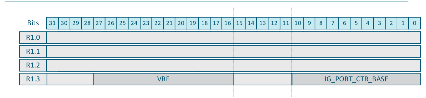
Figure 11. Port metadata register layout

All that's needed now is to populate the ig_port_ctr_base field in the control plane as shown in in the Python script in Figure 12 below:

Figure 12. Sample Python script initializing ig_port_counter_base

1# Program Ingress Port Counter base in the Port Metadata2for port in all_ports:3    set_port_metadata(dev_id, port,4                      PortMetadataValue(vrf=get_vrf(port),5                                        ig_port_ctr_base=port * PACKET_TYPE_MAX))

Going forward, we'll use this method, since it is more general and is somewhat faster as well, not to mention that no code to calculate ig_port_counter_base will be required in the program.

Setting packet_type according to the validation checks

Let's review the IPv4 header validation code that we wrote previously.

Figure 14. Original IPv4 validation code

1v1    BRBTSTCLR    R11.3, 1, not_ipv4_packet2v2    CMPI         R4.0, 28, 4, 43v3    BRINEQ       ipv4_version_invalid4v4    CMPI         R4.0, 24, 5, 45v5    BRILT        ipv4_ihl_invalid6v6    SUBI.F       R0.1, R4.2, 24, 8, 17v7    BRILE        ipv4_ttl_too_small8v8    SYNC.N       2, bad_ipv4_checksum9v9    ###### Fall through to handle valid IPv4 packets10h1    not_ipv4_packet:11h2    ipv4_version_invalid:12h3    ipv4_ihl_invalid:13h4    bad_ipv4_checksum:14h5    ipv4_ttl_too_small:15      …16d1    drop_and_halt:17d2    SYNCALL      25518d3    DROP.H       0

We see that the validation logic is concentrated in lines v1..v8.

Upon any error, the code jumps to one of the labels (lines h1..h5) and then falls through to perform packet dropping.

This means that we can leave the actual validation code intact and simply insert the code that will set the proper packet type and increment the counter just before dropping the packet.

Our new code will look like this:

Figure 15. Accounting for the IPv4 header validation results

1v8    SYNC.N       2, bad_ipv4_checksum2v*    BRI          ig_port_count    # use PACKET_TYPE_GOOD_IPV43h1    not_ipv4_packet:4c1        MOVI     R0.0, 1          # packet_type = PACKET_TYPE_NON_IPV45c2        BRI      ig_port_count6h2    ipv4_version_invalid:7          MOVI     R0.0, 2          # packet_type = PACKET_TYPE_NON_IPV48          BRI      ig_port_count9h3    ipv4_ihl_invalid:10          MOVI     R0.0, 3          # packet_type = PACKET_TYPE_IPV4_BAD_IHL11          BRI      ig_port_count12h4    ipv4_ttl_too_small:13          MOVI     R0.0, 4          # packet_type = PACKET_TYPE_IPV4_BAD_TTL14          BRI      ig_port_count15h5    bad_ipv4_checksum:16          MOVI     R0.0, 5          # packet_type = PACKET_TYPE_IPV4_BAD_CHKSUM17c3    ig_port_count:18c4        ADD.SH   R0.2, R1.3, 0, 11, R0.0, 0, 1119c5        COUNTER  RN, R5, R0.2, 4, 8, 220c6        CMPI     R0.0, 0, 0, 421c7        BRINEQ   drop_and_halt22v9    ###### Fall through to handle valid IPv4 packets23d1    drop_and_halt:24d2        SYNCALL  25525d3        DROP.H   0

Let us discuss it section by section.

First, we can see that the code after each label, corresponding to various failed checks has now been populated by two instructions:

• Line c1: MOVI R0.0, 1: This instruction sets the desired value of the packet type, as per Table 1. Essentially this instruction is identical to the one in line i1 in Figure 13. Register Initialization with the only difference being the actual value being set. The same code is also used after all other labels in lines h2..h5.
• Line c2: BRI ig_port_count: After setting the proper value for the packet type, we jump using the BRI (BRanch Immediate) instruction back to the common code where we will perform the counter increment.
• Line c3: ig_port_count:: This label marks the point where we continue performing the common processing.
• Line c4: ADD.SH R0.2, R1.3, 0, 11, R0.0, 0, 11: This instruction adds together the ingress port counter base (it is located in register R1.3 starting from bit 0 and occupies 11 bits, according to Port Metadata Register Layout) and the packet type that the previous instructions put into register R0.0 (it also occupies 11 bits, starting from bit 0). The result is placed in register R0.2. The .SH (SHort) option suffix indicates that we want to use the faster, 16-bit-wide operation, since our 11-bit-wide operands do not need full 32-bit-wide addition.
• Line c5: COUNTER RN, R5, R0.2, 4, 8, 2: This line forms the heart of our program by incrementing the chosen counter in the IG_PORT_CTR table. First, let's take a look at the last three operands (4, 8, 2). They specify that the instruction must increment a pair (2) of 8-byte-wide counters in the counter table with the ID equal to 4, which is precisely the ID we chose for the IG_PORT_CTR table as per Figure 4. The instruction's second operand (R5) specifies which register is used to increment the counter. As you may recall, we initialized R5.1 with 1 (see Figure 13. Register Initialization), meaning that for now we will only increment the number of packets, while the number of bytes remains 0. The instruction's third operand (R0.2) specifies the location of the counter index that the instruction will be using and we just computed using the previous instruction (line c4). The very first operand is not used by this instruction and thus uses a special dummy register (RN).
• Line c6: CMPI R0.0, 0, 0, 4: After performing the common processing we need to decide whether to continue waiting for the results of the destination lookup or to drop the packet and finish the processing. To do that, we use the CMPI (CoMPare Immediate) instruction to compare the packet type (stored in the register R0.0) to 0, which represents PACKET_TYPE_GOOD_IPV4.
• Line c7: BRINEQ drop_and_halt: The BRINEQ (BRanch Immediate if Not EQual) instruction jumps to the drop_and_halt label in case the value of R0.0 (packet_type) is not equal to 0, bringing the flow execution to the very end of the code where the program handles the invalid packets by dropping them. If, on the other hand, the packet type was equal to 0 (PACKET_TYPE_GOOD_IPV4) then we would have continued the execution moving on to waiting for the results of the IPv4 LPM lookup and sending the packet out.
• Line v*: BRI ig_port_count: This Branch Immediate instruction is needed for good IPv4 packets. Instead of falling through and therefore setting an incorrect packet type, we simply jump around that error handling code straight to the counter increment, since the packet type was already initialized in the beginning of the code.

Accounting for IPv4 LPM hits and misses

We could have followed the same model and added the code used to increment the counters for the packets that hit or missed the IPv4 LPM table. However, we will demonstrate a slightly different coding style that will allow us to slightly speed up the most important case, i.e. the one where we forward the packets.

Figure 16. Accounting for the IPv4 LPM lookup results

1 5    SYNC.N            32, ipv4_lpm_miss2 6    AQMEG.LF3.NOMIRR  R1.0, R3.33m1    ADDI.SX.SH        R0.2, R1.3, 0, 11, 64m2    COUNTER           RN, R5, R0.2, 4, 8, 25 7    MOVI              R3.2, 06 8    MOVI.CD           R0.3, 07 9    SYNC              8810    BRBTSTSET         R1.0, 0, aqm_drop911    SENDOUT.H         R3, R0, 01013    ipv4_lpm_miss:11m3        ADDI.SX.SH    R0.2, R1.3, 0, 11, 712m4        COUNTER       RN, R5, R0.2, 4, 8, 213m5        BRI           drop_and_halt

• Lines 5..6: represent the original code from our previous program. The SYNC.N instruction in line 5 waits for the completion of the lookup in the IPv4_LPM table and jumps to the ipv4_lpm_miss label in case the entry corresponding to the packet's destination IPv4 address was not found in the table. In (the likely) case of a hit, the code falls through to line 6 and initiates the AQM Query.
• Line m1: ADDI.SX.SH R0.2, R1.3, 0, 11, 6: The ADDI (ADD Immediate) instruction computes the new index in the ingress port counter table, corresponding to the PACKET_TYPE_IPV4_LPM_HIT (6). It adds this immediate constant to the ig_port_ctr_base (located in R1.3, starting from bit 0 and occupying 11 bits) and stores the result in the ingress port counter index (still located in R0.2).
• Line m2: COUNTER RN, R5, R0.2, 4, 8, 2: This instruction is exactly the same as the one we previously used in line c5 in Figure 15 incrementing the chosen counter.
• Lines 7..11: These lines also represent the rest of the original code from the previous program. They are responsible for sending the packet out and halting the MAP program.
• Lines m3..m4: These lines are reached only if a miss was encountered in the IPV4 LPM table. They are identical to lines m1 and m2 – the only difference being that the constant added to the base ingress port counter index is equal to 7 (PACKET_TYPE_IPV4_LPM_MISS).
• Line m5: This line is the same as line c7 in Figure 15. It completes processing an IPV4 LPM miss packet by taking it to the common code where it is dropped and the MAP program halted.

Counting packet bytes

So far, we only counted the number of packets corresponding to various conditions (or packet types). While adding this capability has greatly enhanced the program, it would be very useful if we could also count the number of bytes in those packets.

To do that we need to know how long each packet is and the answer to this question is not simple. High-speed switches often start processing packets long before their length is known. This happens because the standard Ethernet-II header (used to carry most of the traffic in modern networks) lacks an explicit packet length indication. As a result, the packet length is determined only later, when the MAC finishes receiving the frame. In many cases, the MAP might already finish processing a jumbo packet, while the MAC continues receiving the tail of the same packet.

XISA devices provide the data plane programmer with two fundamental mechanisms to calculate the packet length:

• Method 1: Many protocol headers do have a field that represents the packet length. For example, IPv4 has the "total_length" field that contains the length of the given datagram. The "payload_length" field in IPv6 headers serves the same purpose. As long as the protocol header is correct, the data plane program can use it to derive the total packet length.
• Method 2: XISA also provides a special SIZEQUERY instruction that can asynchronously report the actual packet length. This mechanism is very helpful when processing the protocols without a proper length field.

We will use the first method to calculate the length of IPv4 packets that passed header validation (corresponding to GOOD_IPV4, IPV4_HIT and IPV4_MISS packet types) and we'll use the second method to calculate the length of all the packets that do not have a valid IPv4 header. Even though that method is slower, it should not affect our program performance, since we are going to use it only for the error cases and (by extension) only for the packets that we intend to drop.

To use the first method, we can use the IPv4 total_length field which is located in bits 15:0 of register R4.0 (see Figure 2 in the previous post). However, to know the full length of the packet, we need to know the offset of the IPv4 header from the beginning of the packet. This can be easily calculated if we remember that register R12 contains the offsets of the individual headers.

Here is how we can calculate the total length of a packet with the valid(ated) IPv4 header using a single instruction that can be added right after the code that checks the validity of IPv4 checksum:

Figure 17. Calculating packet length by using the IPv4 “total length” field

1      SYNC.N    2, bad_ipv4_checksum2L1    ADD       R5.3, R4.0, 0, 16, R12.0, 16, 83      BRI       ig_port_count

• Line L1: ADD R5.3, R4.0, 0, 16, R12.0, 0, 8: We use the ADD instruction to add together the IPv4 "total length" field (it occupies 16 bits starting from bit 0 in register R4.0, see operands 4, 3 and 2) and the IPv4 header offset (stored in the HDR_OFFSET0 register (R12) in byte 1, starting from bit 16 of the sub-register R12.0). The result is placed in register R5.3 which holds the ctr_delta_bytes.

Note how powerful the ADD instruction is. It lets us add values of different widths — while IPv4 total length is a 16-bit field, the IPv4 header offset is only 8 bits wide!

Calculating the packet lengths without a valid IPv4 header is optional – if we do not do it, the program will just count the number of packets. This is another powerful feature of XISA architecture: even though we use pairs of counters we are under no obligation to increment both of them.

Nevertheless, let's demonstrate this code for completeness:

Figure 18. Calculating the size of a non-IPv4 packet

1Q1    SIZEQUERY.LF0    R5.32Q2    SYNC             1

• Line Q1: SIZEQUERY.LF0 R5.3: The SIZEQUERY instruction executes asynchronously. Once it finishes executing, it will place the length of the current packet into the specified destination register. In our case, that's register R5.3 that holds the value of ctr_delta_bytes. The .LF0 option suffix specifies the completion flag used to wait for instruction completion.
• Line Q2: SYNC 1: This instruction waits for the LF0 flag (bitmask is 1) to indicate completion.

XISA is capable of handling much more sophisticated networking tasks. Any standard routing and/or bridging feature, and more importantly, any other unique or customer-driven feature can be implemented thanks to the X-Switch's extreme flexibility and programmability.

For more information, contact us.

We, at Xsight Labs, believe this transparency will drive innovation and facilitate the development of future networking technologies.

Stay tuned for further insights into the capabilities of the X-Switch ISA and the exciting possibilities it unlocks.

The complete MAP program

This is the finished program, with every change from this article applied. The figures above are snapshots taken along the way, so assembling them in order will not produce a working program — use this listing.

1ingress:2      CONCAT.CD         R2.2, 0, R1.3, 16, 123      LKPLPM.LF5.R      R3.3, R3.3, -1, -1, R2, R2, 0, 44i1    MOVI              R0.0, 05i2    MOVI.CD           R5.1, 16      BRBTSTCLR         R11.3, 1, not_ipv4_packet7      CHKSUMTST.LF1     18      CMPI              R4.0, 28, 4, 49      BRINEQ            ipv4_version_invalid10      CMPI              R4.0, 24, 5, 411      BRILT             ipv4_ihl_invalid12      SUBI.F            R0.1, R4.2, 24, 8, 113L1    BRILE             ipv4_ttl_too_small14      SYNC.N            2, bad_ipv4_checksum15      ADD               R5.3, R4.0, 0, 16, R12.0, 16, 816v*    BRI               ig_port_count17not_ipv4_packet:18c1    MOVI              R0.0, 119c2    BRI               ig_port_count_bad20ipv4_version_invalid:21      MOVI              R0.0, 222      BRI               ig_port_count_bad23ipv4_ihl_invalid:24      MOVI              R0.0, 325      BRI               ig_port_count_bad26ipv4_ttl_too_small:27Q1    MOVI              R0.0, 428Q2    BRI               ig_port_count_bad29bad_ipv4_checksum:30      MOVI              R0.0, 531ig_port_count_bad:32      SIZEQUERY.LF0     R5.333      SYNC              134c3    ig_port_count:35c4    ADD.SH            R0.2, R1.3, 0, 11, R0.0, 0, 1136c5    COUNTER           RN, R5, R0.2, 4, 8, 237c6    CMPI              R0.0, 0, 0, 438c7    BRINEQ            drop_and_halt39      STH.SYNC          R0.1, 1, 8, 140      CHKSUMUPD.LF1     141      SYNC              242      SYNC.N            32, ipv4_lpm_miss43      AQMEG.LF3.NOMIRR  R1.0, R3.344m1    ADDI.SX.SH        R0.2, R1.3, 0, 11, 645m2    COUNTER           RN, R5, R0.2, 4, 8, 246      MOVI              R3.2, 047      MOVI.CD           R0.3, 048      SYNC              849      BRBTSTSET         R1.0, 0, aqm_drop50      SENDOUT.H         R3, R0, 051m3    ipv4_lpm_miss:52m4    ADDI.SX.SH        R0.2, R1.3, 0, 11, 753m5    COUNTER           RN, R5, R0.2, 4, 8, 254aqm_drop:55drop_and_halt:56      SYNCALL           25557      DROP.H            058host_eth:59host_pss:60exception:61loopback:62parser_congestion:63trap:64      DROP.H            0

Notes

1. For now, we'll just count the packets. We'll add byte counters later.
2. XISA also provides the ability to decrement and/or set counters atomically; and to even return their values, but we are not going to use these features in this article.
3. If you immediately imagined Mc, M+, M- and Mr buttons available on your calculator, you are absolutely correct!
4. In systems with RMT architecture, the tables and counters are stage-local. Thus, the counter can only be accessed in the stage where it is instantiated, and each packet passes through a stage only once. In systems with dRMT architecture, the memory is global and can, indeed, be accessed from any stage. However, each specific object allocated in such globally accessible memories can usually be accessed from only one stage (although that specific stage is not fixed and determined during program compilation). Doing otherwise requires multi-ported memories or special access serialization techniques (e.g., request queues), which are relatively expensive and can slow down processing.
5. Many other network-oriented instruction sets do not offer such an instruction because it takes a relatively long time to execute, while it is rarely needed for data plane processing.

XISA (the X-Switch Instruction Set Architecture) is Xsight Labs' open instruction set for programming packet processing on the X-Switch family, published under the Mozilla Public License version 2. Programs run across two stages: a Programmable Parser that identifies packet headers, and a Match-Action Processor (MAP) that performs lookups, edits and forwarding.