Simple IPv4 forwarding on XISA™

A peek under the hood: IPv4-based switching using the X-Switch ISA

We're glad to see that our network enthusiasts are back for more. Remember our last deep dive into the nuts and bolts of a network cross-connect? Well, buckle up, because we're back for another peek under the hood! This time, we're tackling something a little more involved, yet super insightful: a basic IPv4 switching program built using the X-Switch Instruction Set Architecture (XISA). This latest example will set you straight regarding what makes network traffic zip along from point A to B.

First, let's define the functionality: our trivial IPv4 switching program will parse the packets, arriving at an ingress port, and continue to forward IPv4 packets to a specified egress port based on the result of the Longest Prefix Match (LPM) lookup of the packet's Destination IP address (DIP) field. For a more realistic LPM lookup, we'll add port-based Virtual Routing and Forwarding (VRF) functionality, meaning that each port can be assigned to a specific routing domain. This program will drop all non-IPv4 packets.

To make things even simpler, we're leaving out several steps typically associated with IPv4 processing, which the current program will not be performing:

1. IPv4 header validation (including IPv4 checksum validation)
2. Time-to-Live (TTL) field validation and decrement
3. Packet header modifications, including Ethernet header rewriting/replacement and IPv4 checksum update.

New in this example, this program will introduce X-Switch packet header parsing concepts, as well as how to perform lookups in explicitly defined tables.

The basic plan

In order to perform an IPv4-based lookup, the program must first parse the incoming packet, that is, identify the specific headers that the packet contains; this is performed by the X-Switch Parser. In addition to identifying the specific headers, the Parser can also preload the values from the selected header fields into the registers that it shares with the X-Switch Match-Action Pipeline (MAP), so that they can be immediately available for further processing in the MAP.^[1]

For example, the Parser program identifies the IPv4 header in the incoming packet and loads the IPv4 Destination Address field into a designated register that is accessible by the Match-Action Pipeline (MAP) program. This preloaded info (i.e. destination IP address in MAP register) is then readily available for the MAP program to use as a key when performing a lookup in a table, such as the IPv4 LPM Forwarding table.

The program also utilizes the built-in Ingress Port Mapping table to implement port-based VRF. The value provided by that table is used as a VRF ID and passed along with the IPv4 destination address to the IPV4 LPM Forwarding table.

The value provided as the result of the LPM Forwarding table lookup is the desired egress queue ID; since, as we learnt in our previous Simple Cross-Connect example, in order to send a packet to a selected egress port, it must be sent to one of the egress queues associated with that egress port. Overall, the algorithm can be graphically represented as shown in Figure 1.

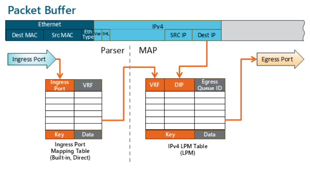
Figure 1. Overall processing diagram

We'll continue to explore the microcode (uCode) in detail in the following sections. Also, see our recently opened XISA for further Instruction details.

Register planning

The parsed header information is passed from the Parser to the MAP using the three registers specifically reserved for this purpose.

MAP register R11, is the HDR_PRESENT register and it contains individual Header Present bits, which the Parser sets as it identifies the corresponding headers inside the packet. This allows the data plane program to work with up to 128 different headers.

Figure 2. MAP register R11: HDR.PRESENT layout

In addition, MAP registers, R12: HDR.OFFSET0 and R13: HDR.OFFSET1, contain 16 slots each to store the individual header offsets, which are expressed as the number of bytes starting from the beginning of the packet. Each offset slot (entry) occupies one byte, meaning that the headers can be located at offsets 0–255 bytes from the beginning of the packet. Using two registers allows the parser to record up to 32 individual header offsets.

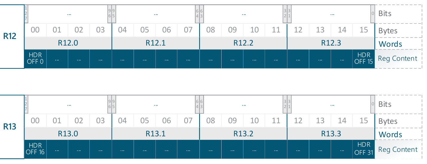
Figure 3. MAP registers R12/13: HDR.OFFSET0/1 layout

Therefore, firstly, we need to enumerate the headers that the program will process along with the layers that they will appear in.

Let's use Table 1 to assign Header ID and Layer ID numbers to the headers in our program. You can use numbers other than 0 and 1, if so desired.

Table 1: Enumerating IPv4 packet headers

Table 2 offers a more complicated case that further illustrates the difference between the Header ID and the Layer ID. Usually, mutually exclusive headers tend to have the same Layer ID, which is why the number of supported Layers (Header Offset IDs) is smaller than the number of Header IDs.

Table 2: A typical header enumeration table

Our next planning step is to decide which header fields to preload into the MAP registers and how to allocate them.

Given that we only need to use the Destination IP Address field from the IPv4 header for the lookup, this is the only field that needs to be preloaded. We can use any spare register for that, such as R2. The 32-bit destination IPv4 address field can be placed anywhere within the R2 128-bit register. We'll go ahead and place it in the least significant bits (Word R2.3), as shown in Figure 4.

Figure 4. MAP register R2 layout: contains destination IP address

Writing the Parser code

Now, let's plan what needs to be done for each of the headers that the Parser is going to identify. The header fields are named in Table 3. Additionally, their offsets (from the start of the header) and their widths (both in bit units) are provided in parentheses.

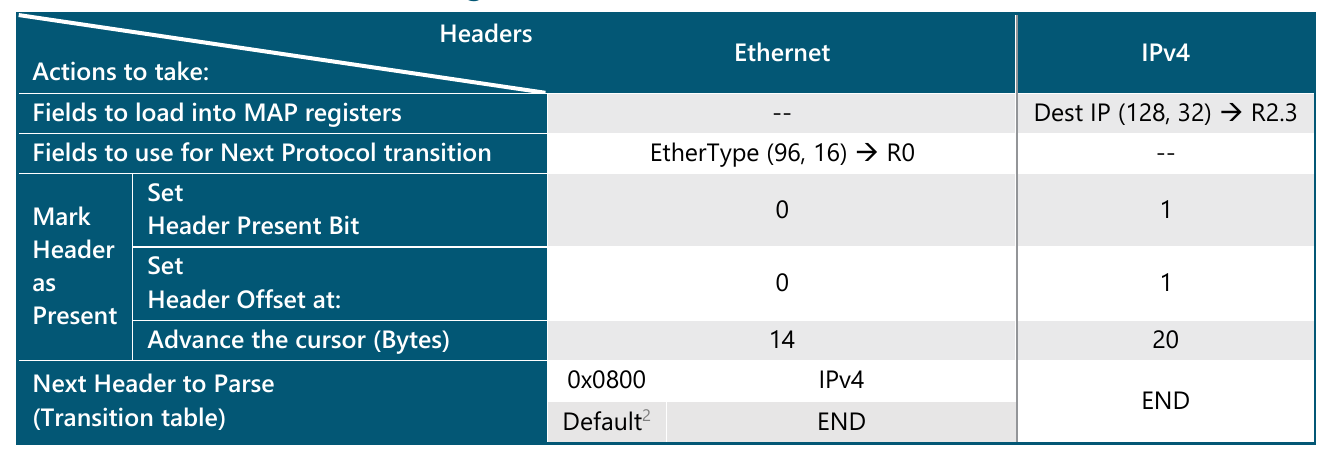
Table 3. Parser header processing

Once the preliminary work has been done, writing the parser code will be very easy.

As always, we start with the initial Jump table that automatically directs the packets to the entry points that correspond to different packet paths. For our example, we're only interested in the ingress packet path that corresponds to regular packets arriving on Ethernet ports. Any specialized packet will simply be dropped as defined in Figure 8.

Figure 5. Parser code. Initial state Jump table

1{2  special_entry_points3    0: ingress:        entry_point_ethernet4    1: reparse:        entry_point_reparse5    2: trap:           entry_point_trap6    3: host_pss:       entry_point_host_pss7    4: loopback:       entry_point_loopback8    5: low_wm:         entry_point_low_wm9    8: hi_wm:          entry_point_hi_wm10}

Next, let's write the code for the initial state and process the Ethernet header according to the details specified in Table 3.

Figure 6. Parser code. Ethernet header parsing (lines 12–19 in the source numbering used by the breakdown below)

1entry_point_ethernet:2    EXTNXTP     R0, 96, 163    {4      entry_point_ethernet5        0: 0x000800: entry_point_ipv46    }7    STHC        14, 0, 0, 18    HALT

Breakdown of these steps

• Line 12: entry_point_ethernet: This label marks the beginning of the processing logic arriving at ingress. The entry points for other packet paths can be found at lines 23 to 28; in all other cases the parsing is terminated, and the packet is dropped.
• Line 13: EXTNXTP R0, 96, 16: The EXTNXTP (EXTract data and calculate NeXT Protocol) instruction loads the data from the packet buffer into a Parser register and then uses its content to choose one of the entries in the transition table. In this particular case the instruction loads the 16-bit EtherType field (located at offset 96 from the beginning of the Ethernet header) into Parser register R0.
• Lines 14–17: These lines represent the transition table associated with the state entry_point_ethernet (as indicated by line 15). The table consists of a single entry to transition to the label entry_point_ipv4 if the content of register R0 is equal to 0x800 (line 16).
• Line 18: STHC 14, 0, 0, 1: The STHC (SeT Header and Cursor position) instruction sets the specified Header Present bit (0) and records the header offset in a given header offset slot (0), according to Table 3. After that, the instruction advances the cursor to the next header by the specified number of bytes (14). The last operand (1) dictates that the instruction transition to the next state (as was previously calculated by the EXTNXTP instruction) or continue to the next instruction (HALT) in case there was no match in the transition table.
• Line 19: HALT: This instruction terminates parsing and is executed when no match is found in the transition table.

Let's continue by writing the code for the state that processes IPv4 headers. The details of this processing have already been planned and described in Table 3.

Figure 7. Parser code. IPv4 header parsing

1entry_point_ipv4:2    EXTMAP      MAPR2, 0, 128, 323    STHC.H      20, 1, 1, 0

• Line 20: entry_point_ipv4: This label marks the beginning of the IPv4 header processing state.
• Line 21: EXTMAP MAPR2^[3], 0, 128, 32: The EXTMAP (EXTract to a MAP register) instruction loads the data from the packet buffer into the MAP register, so that it can be accessed by the Match-Action Processor (e.g. for table lookups). In this particular case the instruction loads the 32-bit Destination IP Address field, located at an offset 128 bits from the beginning of the IPv4 header into bits [31:0] of MAP register R2.
• Line 22: STHC.H 20, 1, 1, 0: This instruction is similar to the one in line 18. This time we update the information for the IPv4 header by setting the Header Present, bit 1, recording the header offset in the Header Offset, slot 1. Then the instruction advances the cursor by 20 bytes (the length of a standard IPv4 header without options). Since there is no need to transition to the next state, the last operand (Jump Mode) is equal to 0, directing the execution transitions to the next instruction. The .H (Halt) option suffix instructs the Parser to stop since this is the terminal state and we have finished the parsing. This suffix is supported by several instructions and saves us from placing an explicit HALT instruction on the next line.

Finally, we'll add trivial code to handle all special packet paths.

Figure 8. Entry points for the special packet paths

1entry_point_trap:2entry_point_host_pss:3entry_point_loopback:4entry_point_reparse:5entry_point_low_wm:6entry_point_hi_wm:7    HALTDROP

• Lines 23–28: These are the entry points for the states that correspond to other packet paths that this program is not designed to handle. They are selected according to the initial Jump table, see Figure 5.
• Line 29: HALTDROP: As can be easily deduced from its mnemonics this instruction halts packet parsing and drops the packet, thereby preventing it from going to the Match-Action Processor.

And that's it! The Parser coding is done; even with the long explanations, the code for each state is short and easy to read.

Writing the MAP microcode

First, let's review our algorithm:

1. Ensure that the packet contains an IPv4 header since the Destination IP address required for the LPM lookup is found only in the IPv4 header. Drop all non-IPv4 packets.
2. Assemble the lookup key by concatenating the required fields in a single register.
3. Perform the table lookup; drop packets upon lookup failures.
4. Check the Active Queue Manager (AQM) to make sure that the packet can be enqueued. If a packet cannot be enqueued, (for example, there may be congestion) drop the packet instead of continuing to send it out.
5. Prepare the operands for the SENDOUT instruction.
6. Send the packet to the chosen Egress Queue.

Next, let's create a register allocation plan. Here is what we know so far:

1. So far, we know that the registers R1, R2, R7^[7], R11, R12 and R13 contain the input from the Parser (see Table 4).
2. We already know that we'll need two full (128-bit-wide) registers to provide the operands for the SENDOUT command. One of them will contain the necessary parameters, including the Egress Queue ID that is expected to be found in Word 3, see Figure 9. The other one just needs to be zeroed out. Since the Egress Queue ID is the result of the lookup in the IPv4 LPM table, it makes sense to try to place that output in the same register where it can be used by the SENDOUT instruction (i.e. in Word 3 of a register).
3. We will need one other word-sized register to hold the output of the AQMEG instruction used to query the queue status.

Table 5 describes register allocations. For each register we first show where it is being written (darker hues) and then, where the value that was written (in the register) is going to be used. We use lighter hues to color all the places where the register needs to hold (carry) the previously assigned value, meaning that it cannot be used for anything else. The vertical arrows show how a value is derived from others.

Compilers often rely on similar data structures to efficiently perform register allocation. In this particular example we chose a straightforward allocation rather than the most optimized one. Zooming in, it's clear that register R1 can be reused to hold everything that was placed in R0 and register R2 can be reused to hold the value for the Advanced SENDOUT parameters that we placed in R3. We'll leave this as an exercise for the reader.

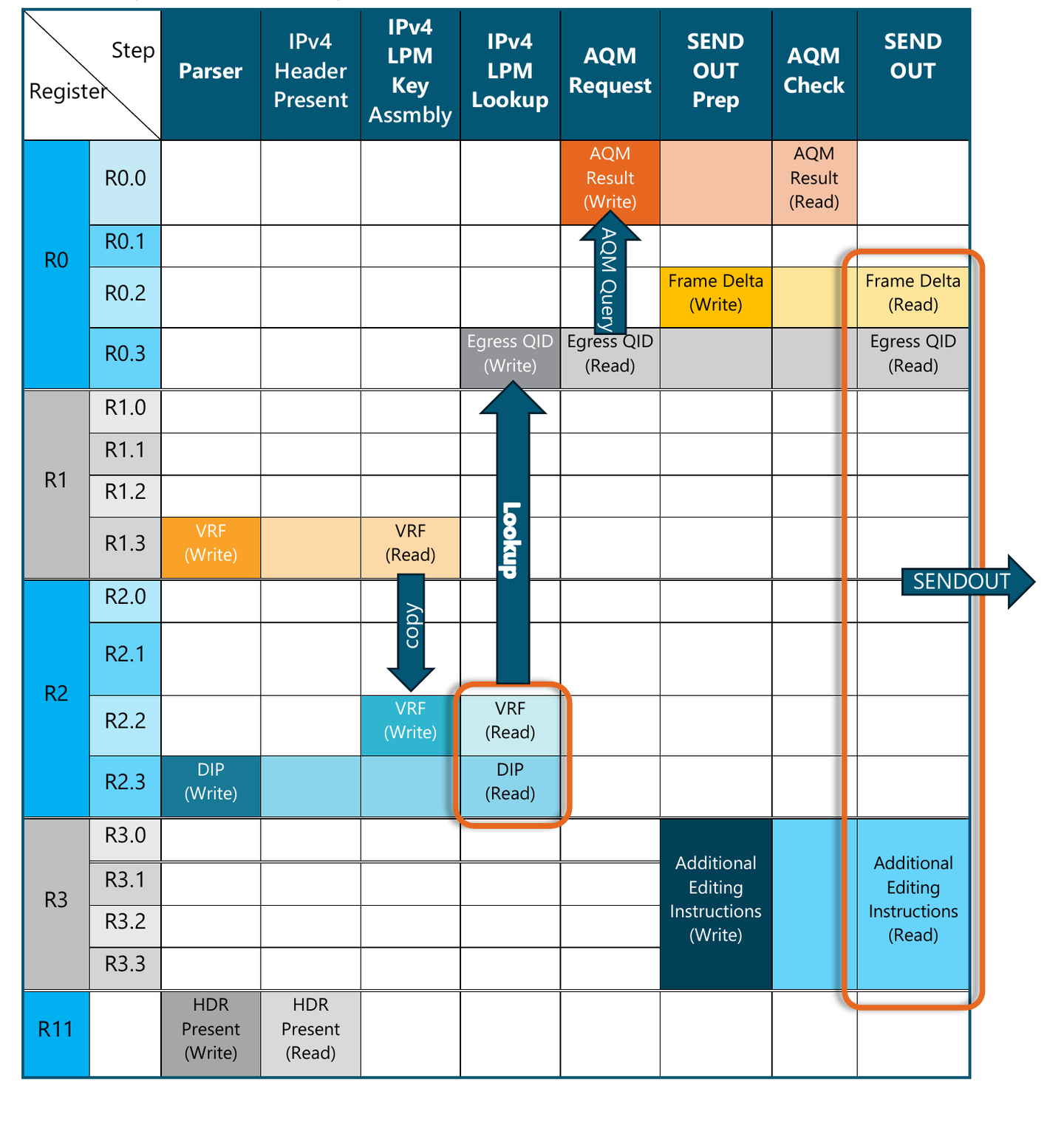
Table 5. Register allocation diagram

Let's get started writing the code:

Figure 12. MAP assembly code

1ingress:2    BRBTSTCLR         R11.3, 1, not_ipv4_packet3    CONCAT.CD         R2.2, 0, R1.3, 0, 124    LKPLPM.LF5.R      R0.3, R0.3, -1, -1, R2, R2, 0, 45    SYNC.N            32, ipv4_lpm_miss6    AQMEG.LF3.NOMIRR  R0.0, R0.37    MOVI              R0.2, 08    MOVI.CD           R3.3, 09    SYNC              810    BRBTSTSET         R0.0, 0, aqm_drop11    SENDOUT.H         R0, R3, 012not_ipv4_packet:13ipv4_lpm_miss:14aqm_drop:15    DROP.H            016host_eth:17host_pss:18exception:19loopback:20parser_congestion:21trap:22    DROP.H            0

Breakdown of these steps

• Line 1: ingress: This pre-defined label name determines the starting point for packet processing in the MAP, upon ingress. The other entry points can be found in lines 18–23.
• Line 2: BRBTSTCLR R11.3, 1, not_ipv4_packet: Recall that register R11 contains the HDR.Present bits (see Figure 2 and Table 4) and we chose bit 1 to represent the presence of the IPv4 header (see Table 1). The BRBTSTCLR instruction (BRanch on Bit TeST CleaR) tests whether bit 1 is cleared in that register and if so, it will perform a Jump to the specified label (not_ipv4_packet). Note that the instruction performs the test within a 4-byte word. Bit 1 is located within Word 3 of register 11 (R11.3), so that's what we're specifying.
• Line 3: CONCAT.CD R2.2, 0, R1.3, 0, 12: The bitwise CONCATenation instruction can concatenate two arbitrary bit-fields or copy one bit-field from one location to another. Thus, this instruction is especially handy for assembling table lookup keys. Given the key definition in xdefs.json file (see Figure 11), we need to prepend the VRF field to the (left of the) Destination IP address (prefix) field. Figure 13 graphically illustrates that process. Note that it is essential to clear the unused bits in register R2.2. This is achieved by appending the CD (Clear Destination) suffix to the instruction.

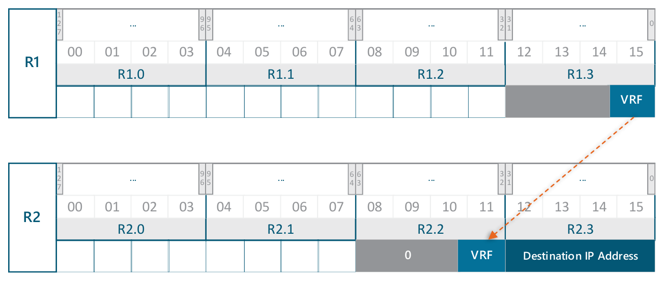
Figure 13. Forming the lookup key for the IPv4_LPM table

• Line 4: LKPLPM.LF5.R R0.3, R0.3, -1, -1, R2, R2, 0, 4: The LKPLPM (LooKuP in LPM table) instruction initiates the table lookup. The first two operands (both being R0.3) indicate the start and the end of the destination, where the result of the lookup should be placed. In our case, the size of the result is 4 bytes (as indicated by the very last operand of the instruction), which is why both the start and end are the same. The result of the lookup can also be returned in a memory instead of a register (or even both); however, the instruction's .R suffix indicates that the result will be returned just in the Register (R0.0). As such, the third and the fourth operands are ignored.
  • The next two operands (R2) provide the location of the key.
  • The penultimate operand (0) is the ID of the IPv4 LPM table, which was defined in the xdefs.h file (see line 24 in Figure 11).

All X-Switch lookup operations execute asynchronously. The device provides eight special bit flags (LF0 through LF7) that are set when an asynchronous instruction completes and thus, can be used for synchronization. The .LF5 suffix indicates that we chose bit LF5 for synchronization with this instruction. Meanwhile, program execution continues in parallel with the lookup.

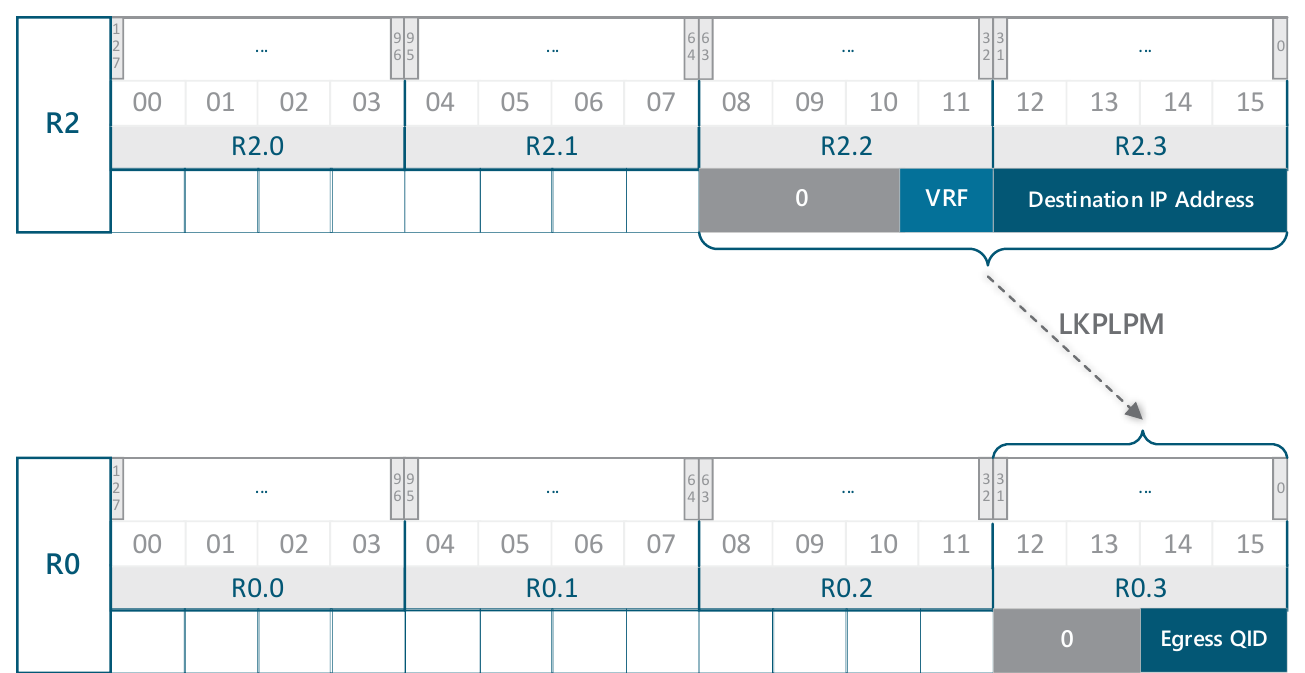
Figure 14. Performing the LPM lookup: key and result (value)

• Line 5: SYNC.N 32, ipv4_lpm_miss: We now need to wait for the lookup operation to complete, which is achieved by using the SYNC instruction. The first parameter specified a bitmap of flags that the code needs to wait on. Since we used the LF5 flag in the LKPLPM instruction, the bitmask must have the 5th bit set in it, which gives us the decimal number 32. The .N (No match) suffix specifies that if there is no match, the code should jump to the label specified as the second operand, ipv4_fib_lpm_loopkup_miss, (see line 14 in Figure 12).
• Line 6: AQMEG.LF3.NOMIRR R0.0, R0.3: Before we send the packet to the output queue, it's good practice to query the Queue Manager (QM) to proactively check if there is space to enqueue the packet. Use the AQMEG (Active Queue Management for EGress) instruction to take the egress queue ID (located in R0.3) as the input and return the result in R0.0 (see Figure 12). Since this is an asynchronous instruction, we'll choose the LF3 flag to wait for instruction completion. We'll also use the .NOMIRR suffix to indicate that there is no need to mirror the packet.
• Line 7: MOVI R0.2, 0: While AQMEG is running, further code execution can continue in parallel. We'll use this time to finish preparing all the registers needed for SENDOUT. Let's also use the MOVI (MOVe Immediate) instruction to populate the Frame Delta field with 0, as defined in Figure 9.

Figure 15. Setting Frame Delta in register R0 (R0.2)

• Line 8: MOVI.CD R3.3, 0: While still waiting for the result of the AQMEG instruction, we need to clear register R3, so that it can be used to provide the Advanced parameters for the SENDOUT instruction (refer to Table 5: Register Allocation Diagram). This specific instruction form is a standard XISA idiom for clearing an entire 128-bit register (which is what we need since we do not plan to pass any additional editing parameters to the SENDOUT instruction). The .CD (Clear Destination) option suffix first clears the entire register (R3) and then moves the immediate operand (in this case 0) into Word 3 of this register.
• Line 9: SYNC 8: Here we use the SYNC instruction to wait for the AQMEG instruction to complete. Since the AQMEG instruction was used with an .LF3 suffix, the newly constructed bitmap is equal to 8. Once the results are ready (in R0.0 as was requested), the execution flow continues with the next instruction.
• Line 10: BRBTSTSET R0.0, 0, aqm_drop: The result, returned by the AQMEG instruction in R0.0 will have bit 0 set in case the packet needs to be dropped. This instruction tests that bit 0 is set and Jumps to the aqm_drop label (see line 15) if set.
• Line 11: SENDOUT.H R0, R3, 0: Finally, we'll send out our packet. The main parameters are contained in register R0 (see Figure 15) and the Advanced Parameters are contained in register R3 (which was set to 0). The third operand (0) specifies that no additional buffers for the packet are required, since the program did not modify it.^[8] The instruction option suffix .H (Halt) stops the packet processing after sending the packet. And we're done!
• Lines 13–16 are responsible for processing various runtime conditions that our program might encounter, such as receiving a non-IPv4 packet, a miss in the IPv4 LPM table or lack of space in the QM. In all those cases the packet is dropped using the DROP.H instruction.
• Lines 18–24: These lines provide trivial handling for other entry points. They are mandatory and thus, must be present in the program. In all these cases the packet will simply be dropped and the program execution halted.

Beyond the simplicity: XISA's potential

This example demonstrates several new features and capabilities of the XISA architecture. We learned how to code a simple parser, how the parsed headers and other data are passed to the MAP, how to plan MAP register allocation, how to create a simple LPM table and finally how to put everything together, all in about 50 lines of code. The bulk of the parsing is achieved using just six instructions. Furthermore, most of the MAP processing is done using only 10 instructions.

XISA is capable of handling much more sophisticated networking tasks. Any standard routing and/or bridging feature, and more importantly, any other unique or customer-driven feature can be implemented thanks to the X-Switch's extreme flexibility and programmability. For more information, contact us.

We, at Xsight Labs, believe this transparency will drive innovation and facilitate the development of future networking technologies.

Stay tuned for further insights into the capabilities of the X-Switch ISA and the exciting possibilities it unlocks.

Notes

1. Fields that were not explicitly loaded in the registers can be retrieved by the MAP from the packet buffer later, but loading the data in the registers makes the program much more efficient.
2. Not part of the actual transition table, see STHC instruction details below.
3. Note that the Parser code MAP registers are specified using the names with a MAP prefix, such as MAPR2, whereas the names with no prefix, such as R0, refer to the internal Parser registers.
4. Because any MAP register can be used as a Parameter Register for the SENDOUT instruction, we indicate that by using the designation "R?" instead of the specific register number.
5. This description is simplified for clarity.
6. The symbol IPV4_LPM_TABLE_ID is defined from the enumerator ipv4_lpm_table in Figure 11. The name of the enumerator is capitalized and the name of the specific value ("id") is also capitalized and appended with an underscore.
7. The registers R7, R12 and R13 are not used by this program, but will be used in more complex ones.
8. This parameter differs from Frame Delta.

XISA (the X-Switch Instruction Set Architecture) is Xsight Labs' open instruction set for programming packet processing on the X-Switch family, published under the Mozilla Public License version 2. Programs run across two stages: a Programmable Parser that identifies packet headers, and a Match-Action Processor (MAP) that performs lookups, edits and forwarding.