A network calculator on XISA™
A baby step towards in-network compute: implementing XCalc
This tutorial implements XCalc, a network calculator on the X-Switch ISA. The Parser recognizes a custom L2 header (Ethertype 0x1234) carrying an opcode and two operands; the MAP looks the opcode up in a table of jump addresses, performs the arithmetic or logical operation, writes the result into the packet, swaps the MAC addresses and returns it to the sender — demonstrating computed branches, loops and in-network compute.
Leaving the world of IPv4 switching
Welcome back, network enthusiasts! Today we decided to leave the world of IPv4 switching and to use XISA to implement a classical example, popularized by a P4 language tutorial, a network calculator, that we will appropriately call XCalc.
The idea is that devices with programmable data planes can do a lot more than just forward packets. For example, they can be used to perform computations using packet fields as data. Back in 2016/2017, this concept was seen as clever, but mostly academic and not very practical. Fast-forward to 2025 and it's gaining serious traction. Today, there's growing interest in using switches to accelerate machine learning, by performing simple, but critical arithmetic operations while switching the packets carrying training data.
This is where X2 switches outshine many competitors, due to their ability to perform just-in-time parsing and arbitrarily complex calculations, that resemble a traditional CPU way more than a switch.
Let's start small. In this example we'll concentrate on the essentials: a simple, table-based switch() statement and some basic arithmetic and logical operations. Think of this as laying the foundation. Once we've got that down, we'll move on to the more advanced stuff.
Defining XCalc functionality
For this simple example we'll use the same packet format as described in the standard P4 language tutorial. It will be a simple L2-based protocol utilizing Ethertype 0x1234. The header will have the following format:

Figure 1. XCalc header (version 1)[1]
where:
- X is an ASCII Letter 'X' (0x58) or 'x' (0x78)
- 2 is an ASCII Digit '2' (0x32)
- Version is currently 0.1 (0x01)
- Opcode is an operation to perform:
Supported opcodes
The switch receives the packet and verifies that it is correctly formed. It continues to perform the specified operation, writes the result into the Result field and then sends the packet back to the same port it came from, while also swapping the Ethernet source and destination MAC addresses.
Later on, we can add more operations and extend the functionality in other ways.
Register planning
Register planning is a critical part of writing a program in any assembly language. Strategically placing the data in the registers can significantly reduce the need for extra data movement or the need to temporarily save the register contents in memory and, hence, speed up the program.
XISA provides fourteen 128-bit-wide general-purpose registers, named R0..R13 in its Match-Action Processor (MAP). Each register can be subdivided into four independent 32-bit registers each. For example, register R0 can be subdivided into registers R0.0, R0.1, R0.2 and R0.3.
As we discussed in our previous articles, the programmable parser can load the most often needed headers or their parts into the MAP registers to speed up the processing. Also, it preloads certain registers with standard information, such as Port Metadata (R1), Standard Metadata (R7.0), Header Present (R11) and Header Offsets (R12..R13), so it's best if we leave these untouched.
Figure 2 illustrates the layout of the headers we are going to use for this exercise:
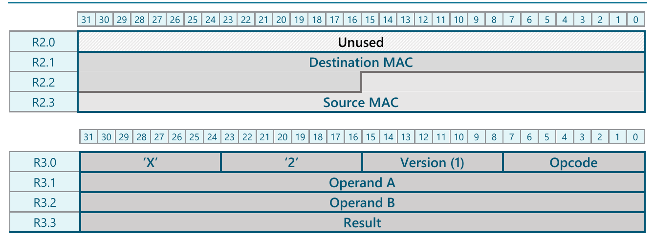
Figure 2. Register layout for the program headers
Parser code
Parsing a custom header, such as the XCALC Header we defined above, is no different than parsing a standard header, such as Ethernet. All we need to do is:
Defining the parse graph
In our case the parse graph can be very simple, as described in Figure 3.
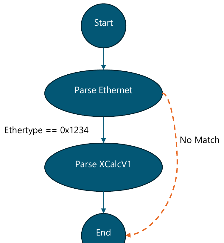
However, we've already future-proofed the header with the signature and the version, potentially allowing for more versions of the XCalc header in the future that can be encapsulated using the same Ethertype (0x1234) if the first three bytes (two-byte signature and one-byte version fields) remain the same. Therefore, let's create a slightly more complex parse graph to allow us to easily add more versions of this protocol in the future. This will also demonstrate that state transitions, header extraction and header recording (that is the process of marking the header "present" and storing its offset) can be completely independent.
Figure 4 shows how the expanded Parse Graph might look:
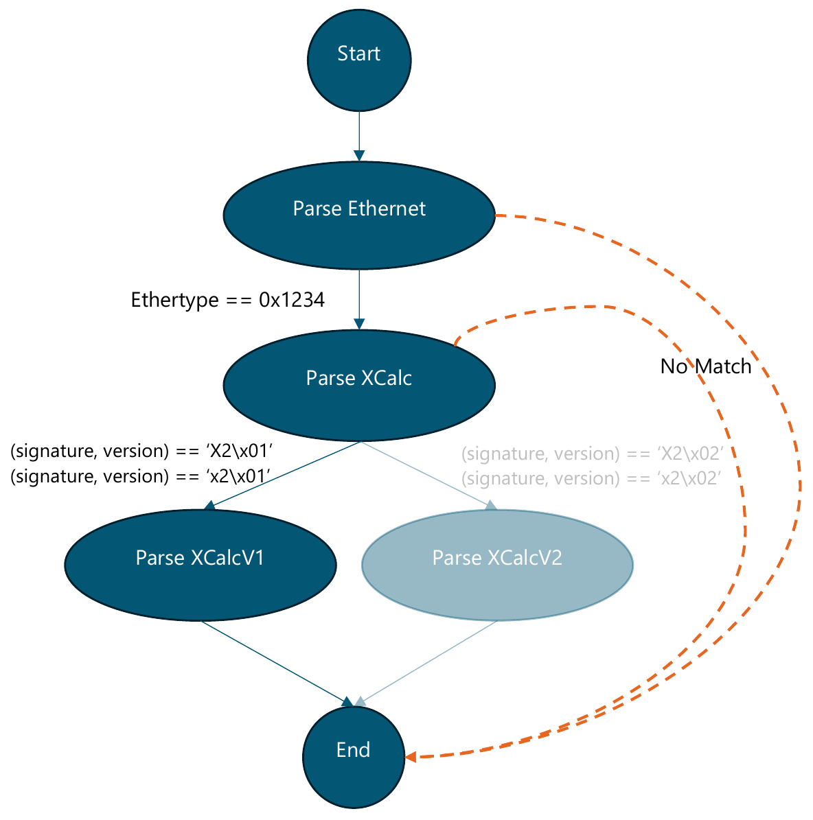
While this graph has one extra transition it allows us to expand the program more easily and to also perform the signature and verification in the Parser which is different, compared to our previous example where we were performing IPv4 version and header length checks in the MAP.
Which method is better? This depends somewhat on the overall structure of the code; the important point is that XISA provides the programmer with the flexibility about where to perform the check.
Allocating Header IDs and Header Offset IDs
We discussed the general algorithm for allocating the Header IDs and Header Offset IDs in one of our previous articles. As a reminder, Header IDs need to be allocated for all distinct headers that the program intends to process, whereas Header Offset IDs need to be allocated for the distinct layers or positions a certain header can occupy in the packet.
In our case, the table can look like this:
Table 1: Allocating Header IDs and Header Offset IDs
Note how the Layer ID is the same for both XCalcV1, XCalcV2, and potentially for other XCalc headers. It is clear from the Parse graph that only one of them can be present in a given packet yet, in all the cases it will follow the Ethernet header.
Writing the Parser code
We'll skip writing the standard preamble, since it was discussed in the previous articles. Instead, we'll concentrate on coding the states that parse the Ethernet header and the XCalc header(s).
Parsing the Ethernet
The goal of this state is to preload the Ethernet Destination and Source MAC addresses into the R2 MAP register as per Figure 2 and perform the transition based on the Ethertype.
Figure 5. Parsing Ethernet
parse_ethernet: EXTMAP MAPR2, 0, 0, 96 EXTNXTP R0, 96, 16 { parse_ethernet 0: 0x001234: parse_xcalc } STHC 14, 0, 0, 1 HALTHere is a detailed breakdown of these steps:
- Line 1: parse_ethernet: This label marks the beginning of the processing logic arriving at ingress.
- Line 2: EXTMAP MAPR2, 0, 0, 96: The EXTMAP (EXTract into a MAP Register) instruction loads the data from the input packet byte stream into the MAP registers. Since the parser has access to both the Parser and the MAP registers, the latter are always specified in the Parser code using the MAPRx notation. This instruction loads 96 bits, starting from bit 0 of the packet (i.e., the destination and the source MAC addresses) into R2 (MAP register) such that the least significant bit (LSb) of the Source MAC address (the last bit to be extracted by this instruction) is placed into R2's LSb (that is, bit 0).
- Line 3: EXTNXTP R0, 96, 16: The EXTNXTP (EXTract data and calculate NeXT Protocol) instruction loads the data from the packet buffer into a Parser register and then uses its content to choose one of the entries in the transition table. In this case the instruction loads the 16-bit EtherType field (located at offset 96 from the beginning of the Ethernet header) into Parser register R0.
Note: The order of these instructions is very important, as it is critical to access the data in the same order it appears in the byte stream.
- Lines 4–7: These lines represent the transition table associated with the state parse_ethernet (see Figure 5, Line 5). The table consists of a single entry to transition to the label parse_xcalc if the content of register R0 is equal to 0x1234 (see Figure 5, Line 6).
- Line 8: STHC 14, 0, 0, 1: The STHC (SeT Header and Cursor position) instruction sets the specified Header Present bit (0) and records the header offset in a given Header Offset slot (0), according to Table 1. After that, the instruction advances the cursor to the next header by the specified number of bytes (14). The last operand (1) dictates that the instruction transition to the next state (as was previously calculated by the EXTNXTP instruction) or continue to the next instruction (HALT) when a match is not found in the transition table. The STHC (SeT Header and Cursor position) instruction sets the specified Header Present bit (0) and records the header offset in a given Header Offset slot (0), according to Table 1. After that, the instruction advances the cursor to the next header by the specified number of bytes (14). The last operand (1) dictates that the instruction transition to the next state (as was previously calculated by the EXTNXTP instruction) or continue to the next instruction (HALT) when a match is not found in the transition table. [[Source says "according to Table 2"; there is only one allocation table on this page — reference corrected to Table 1.]]
- Line 9: HALT: This instruction terminates parsing and is executed only when no match is found in the transition table from the previous instruction.
Parsing the common portion of the XCalc header(s)
Now, we need to extract the next three bytes that should represent the signature and the version fields of the XCalc header (see Figure 1). Not only do we need to extract these three bytes, but we also need to place them into the most significant bits of register R3 as depicted in Figure 2.
To do this we'll use the following technique:
- First, we'll extract this data into a Parser register (e.g., R0) so that we can use it to look up the next state.
- Next, we can copy the data from the Parser register into a MAP register using the MOVMAP instruction, thereby avoiding the double extraction of the same data.
Here is the full code of that state:
Figure 6. Parsing XCalc
parse_xcalc: EXTNXTP R0, 0, 24 MOVMAP MAPR3, 104, R0, 0, 24 { parse_xcalc 0: 0x583201: parse_xcalc_v1 /* 'X2\x01' */ 1: 0x783201: parse_xcalc_v1 /* 'x2\x01' */ 2: 0x583201: parse_xcalc_v2 /* 'X2\x01' */ 3: 0x783201: parse_xcalc_v2 /* 'x2\x01' */ } BRNXTP 1 HALTHere is a breakdown of these steps:
- Line 2: EXTNXTP R0, 0, 24: The EXTNXTP (EXTract data and calculate NeXT Protocol) instruction loads the data from the packet buffer into a Parser register and then uses its content to choose one of the entries in the transition table. Since we had previously moved the cursor past the Ethernet header, the signature and the version fields of the XCalc header are located at Offset 0 and their total bit width is 24 bits. Thus, they will be loaded into the Parser's Register R0 and used to calculate the next state. Important! This instruction always loads the data into the lower bits of the specified register, such that the LSb of the extracted data is placed into the LSb of the register (bit 0).
- Line 3: MOVMAP MAPR3, 104, R0, 0, 24: The MOVMAP (MOVe to a MAP Register) instruction takes the 24 bits located at Offset 0 of Parser Register R0 and copies them into MAP register R3 at Offset 104, meaning that they will be placed in bits [127:104], exactly as specified in Figure 2.
- Lines 4–10: This is the transition table for this state. For illustrative purposes we'll put four possible match values for the (signature, version) combination. Note, that the ASCII characters must be converted into Hex notation. Lines 8 and 9 (Figure 6) are not necessary for this example, but can be added later if we decide to expand the program to process the next version of the protocol.
- Line 11: BRNXTP 1: The BRNXTP (BRanch to the NeXT Protocol) instruction performs the transition (jump) to the next state (calculated by the EXTNXTP instruction) without advancing the parser cursor and/or recording the presence of the header or its offset. This will be done in the next state(s) when we know which header we are extracting. To put it another way, this instruction allows us to implement a lookahead. The sole operand of the instruction (1) specifies that if a mismatch in the transition table is found, execute the next instruction (HALT).
- Line 12: HALT: This instruction terminates parsing and is executed when no match is found in the transition table. Note, that if that happens, MAP register R3 still contains the first three bytes of the header, but no additional Header Present bits beyond the Ethernet one will be set.
Parsing the XCalcV1 header
Assuming that the signature of the header is correct (X2 or x2) and the version is equal to 1, we are now at the point where we need to extract the XCalcV1 header. Since the first 3 bytes have already been extracted and placed into the top 3 bytes of MAP register R3, all we need to do is to extract 13 more bytes (since the total length of the header is 16 bytes) and then advance the cursor and record the header presence and offset.
Figure 7. Parsing XCalc_V1
parse_xcalc_v1: EXTMAP MAPR3, 0, 24, 104 STHC 16, 1, 1, 0 HALTHere is a breakdown of these steps:
- Line 2: EXTMAP MAPR3, 0, 24, 104: This instruction is very similar to the one that we used to extract the Ethernet Destination and Source MAC addresses. In this case, the offset in the packet is specified as 24 bits, since we didn't advance the cursor in the previous step and the first extracted field (Opcode) is located at offset 24. The total number of extracted bits is 104 (13 bytes) and they will be placed into MAP register R3 at Offset 0, leaving the upper bits that already contain the beginning of the header intact.
- Line 3: STHC 16, 1, 1, 0: The STHC (SeT Header and Cursor position) instruction sets the specified Header Present bit (1) and records the header offset in a given header offset slot (1), according to Table 1. After that, the instruction advances the cursor to the next header by the specified number of bytes (16). Since we didn't perform any lookup in the transition table, we simply need to continue to the next instruction, which is what the last operand (0) specifies.
- Line 4: HALT: The instruction terminates parsing.
MAP code
The processing code for the XCalcV1 packets that we are going to write includes the following steps:
- Verifying the presence of the XCalcV1 header by checking the corresponding HDR_PRESENT bit.
- Performing the (asynchronous) lookup in the opcode table that will map each supported opcode into the corresponding jump point in the program.
- While lookup is proceeding, we can swap the source and destination MAC addresses in the packet.
- Once the lookup is done, we can jump to the point in the program that will perform the requested operation (addition, subtraction, etc.).
- After the desired operation has been performed, the result needs to be placed in the packet.
- The last step would be to send the packet out to the same port it came from. This is done by employing the Port Metadata table in the same way that was discussed in the Simple Cross-Connect example.
Let's have a closer look at those steps.
MAP input
Let's review the input the MAP receives from the Parser.
Table 2: MAP input from Parser [[Source captions this "MAP Input to Parser"; corrected to match the sentence above and the other tutorials.]]
Defining the OPCODE table
The X2 match tables are very flexible and this is reflected in XISA. The details of the tables, such as their size, placement, etc., are abstracted from the table lookup instructions using the concept of Table IDs, an integer assigned to each table during its provisioning.
For this reason, the Tables are defined separately from the assembly code, using two JSON files. The first file, xdefs-tables.json specifies the Tables used by the given program on a high level.[2]
Figure 8. xdefs-tables.json OPCODE table definition
{ "table": [ { "name": "OPCODE", "id": "OPCODE_TABLE_ID", "type": "Hash", "size": 256, "key_size": 8, "key": "OpcodeKey", "value": "OpcodeValue" }The second file, xdefs.json specifies the layout of the Table entry (both Key and Value) as well as defines the Table ID.
Figure 9. xdefs.json defining the layout of the OPCODE table, key and value
{ "struct": [ { "name": "OpcodeKey", "description": "Opcode Table Key (Opcode character)", "fields": [ { "type": "BitField", "name": "opcode", "size": 8, "value": 0 } ] }, { "name": "OpcodeValue", "description": "Opcode Table Value (jump label)", "fields": [ { "type": "BitField", "name": "valid", "size": 1, "value": 0 }, { "type": "BitField", "name": "padding", "size": 23, "value": 0 }, { "type": "BitField", "name": "jump_address", "size": 32, "value": 0 } ] }, ],
"enumerator" : [ {"name": "opcode_table", "values": [ {"name":"id", "value": 5} ] } ]}As can be seen from the definition above, the OPCODE table Key is the 8-bit opcode (that will come directly from the XCalcV1 header) and the Value is the 32-bit jump address that will be programmed to point to the code that executes the operation, specified by the opcode.
Let's see how this works in the code.
Using the OPCODE table and performing the operations
The code that checks the presence of the XCalcV1 header (Figure 10), initiates the lookup in the OPCODE table and performs the jump according to the received value.
Figure 10. Using the OPCODE table for jump address selection
ingress: BRBTSTCLR R11.3, 1, not_xcalcv1_packet LKP.LF0.R R0.0, R0.0, -1, -1, R3.0, R3.0, 5, 1, 1, 4 SYNC.N 1, unknown_opcode BR R0.0
do_add: ADD R3.3, R3.1, 0, 32, R3.2, 0, 32 BRI calc_donedo_sub: SUB R3.3, R3.1, 0, 32, R3.2, 0, 32 BRI calc_donedo_and: AND R3.3, R3.1, 0, R3.2, 0, 32 BRI calc_donedo_or: OR R3.3, R3.1, 0, R3.2, 0, 32 BRI calc_donedo_xor: XOR R3.3, R3.1, 0, R3.2, 0, 32 BRI calc_done
calc_done:Here is a breakdown of these steps:
- Line 1: ingress: This is a standard name for the MAP entry point for the regular packets, received from an Ethernet port.
- Line 2: BRBTSTCLR R11.3, 1, not_xcalcv1_packet: We use the BRBTSTCLR (BRanch on Bit TeST CLeaR) instruction to test bit 1 in register R11, which is the Header Present bit corresponding to the XCalcV1 header. If the bit is clear, the program execution will continue at the address not_xcalcv1_packet, where it will be dropped. Since the instruction can only operate on 32-bit register words, we cannot specify the whole 128-bit-wide register (R11). Instead we specify the word-register (R11.3) where bit 1 is located.
- Line 3: LKP.LF0.R R0.0, R0.0, -1, -1, R3.0, R3.0, 5, 1, 1, 4: The LKP (LooKuP) instruction performs asynchronous lookup in the specified table. The table ID (5) is specified as the 7th operand. Because the Table Keys and Values can be quite wide, they might be placed in multiple registers. The first two operands of the command specify the first and the last register that will contain the value, whereas the last operand (4) specifies the number of bytes that should be returned. In our case, a one word-sized register (R0.0) will suffice, since the jump addresses are 32-bits wide. The third and fourth operands (-1) are ignored and the two operands that follow (R3.0) specify the start and the end register that contain the Key. In our case, the Key is contained in register R3.0 in bits 7:0. The width of the key is specified using the two operands that follow the Table ID (1, 1). The first of them specifies the width of the Key, while the second defines the units (1 indicating bytes).
- Line 4: SYNC.N 1, unknown_opcode: The SYNC instruction waits for the asynchronous instructions to complete using a bitmap of flags to wait on. Since the LKP instruction used the LF0 flag, we set bit 0 in the bitmap, which results in the value 1. The option suffix .N indicates that we also want to provide an address to jump to in case there was no match in the Table. The second operand is the label specifying the jump address for a lookup miss (Line 15 in Figure 11).
- Line 5: BR R0.0: This is the key to the solution! The BR (BRanch) instruction performs a jump to the address specified in its first operand, which is a register (R0.0) and if you remember, the value in it, is the result of the lookup in the OPCODE table! This is fundamentally different from the BRI (BRanch Immediate) instruction that we used in all previous examples where the jump address was a literal (label) specified in the compile-time.
- Line 7: do_add: This is one of the labels, the address of which is going to be programmed in the OPCODE table in the entry with the ASCII '+' (0x2b) as a key.
- Line 8: ADD R3.3, R3.1, 0, 32, R3.2, 0, 32: The ADD instruction adds together OperandA (located in R3.1) and OperandB (located in R3.2) and places the result in the result field (R3.3). The additional two pairs of operands specify the bit offset (0) and the width (32 bits) of the actual operands within their respective registers. The result of this instruction is always 32-bit wide and thus occupies the entire R3.3.
- Line 9: BRI calc_done: This BRI (BRanch Immediate) instruction performs the jump to the calc_done label where we'll continue the common processing, such as swapping the MAC addresses, updating the packet with the result and sending it out.
- Lines 10–21: These lines follow the same pattern as Lines 7–9. Note that the operand width for the logical instructions is specified only once, since it is the same for both operands.
Updating and sending the packet
Now that the required arithmetic or logical operations have been performed, we need to update the packet and send it out, specifically:
- Swap the Destination and Source MAC addresses.
- Write the result into the packet buffer.
- Send the packet out.
Here is how this can be implemented:
Figure 11. Updating and sending the packet
calc_done: STH R2, 0, 0, 6 SHRI R2, R2, 0, 96, 48 STH R2, 0, 6, 6
STH.SYNC R3.3, 1, 12, 4
AQMEG.LF1.NOMIRR R0.0, R1.3 MOVI.CD R2.3, 0 SYNC 2 BRBTSTSET R0.0, 0, aqm_drop SENDOUTI.H R1, R2, 0, 0
not_xcalcv1_packet:unknown_opcode:aqm_drop: SYNCALL 255 DROP.H 0Here is a breakdown of these steps:
- Line 2: STH R2, 0, 0, 6: The STH (STore in the Header buffer) instruction stores the data from the register (R2) into the section of the header buffer, identified by the header offset ID (0) with the additional byte offset (0). The header offset 0 corresponds to the Ethernet header (see Table 1) and offset 0 corresponds to the Destination MAC address. The 6 lower bytes in register R2 contain the Source MAC address as it was extracted by the Parser (see Figure 2). As such, this instruction writes the Source MAC address of the packet in the location where the destination MAC address should be.
- Line 3: SHRI R2, R2, 0, 96, 48: The SHRI (SHift Right Immediate) instruction shifts the 96 lower bits of register R2 (bits 95:0) by 48 bits to the right. As a result, the original Source MAC address gets pushed out and R2's lower 48 bits (6 bytes) are now occupied by the Destination MAC address (see Figure 2).
- Line 4: STH R2, 0, 6, 6: The STH (STore in the Header buffer) instruction stores the data from the register (R2) into the section of the header buffer, identified by the header offset ID (0) with the additional byte offset (6). The header offset 0 corresponds to the Ethernet header (see Table 1) and offset 6 corresponds to the Source MAC address. After the shift, register R2's 6 lower bytes now contain the Destination MAC address. As such, this instruction writes the Destination MAC address of the packet in the location where the Source MAC address should be.
- Line 6: STH.SYNC R3.3, 1, 12, 4: We use the STH instruction again, this time to store the XCalc result located in R3.3 (see Figure 2) into the header buffer. In this case, we use Header Offset ID 1, which corresponds to the XCalcV1 header, with the additional 12 byte offset, corresponding to the Result field. The total number of bytes to store is indicated in the last operand of the instruction (4). This instruction also uses the .SYNC option suffix to ensure that the execution of the next instruction starts only after all writes into the packet buffer have been completed.
- Lines 8–12 are used to send the packet out (code was detailed in our previous articles). The only difference here is in the specific register numbers.
- Lines 14–18 are used to drop the packet in case we run into any error or if a run-time condition (Queue Full) is encountered. This code was also discussed before.
This concludes our basic project.
Additional modifications
Now that we have the basic infrastructure in place, it becomes easy to add more operations to our calculator. Here are some we would suggest as an exercise to the interested readers.
Here are examples of additional useful operations that can be implemented using a single instruction available in XISA followed by a branch to calc_done:
- Result = OperandA << OperandB
- Result = OperandA >> OperandB
- Result = OperandA % OperandB
- Result = RandomNumber()
Here are examples of additional useful operations that can be implemented using a simple sequence of instructions, for example:
- Result = min(OperandA, OperandB)
- Result = max(OperandA, OperandB)
In addition, it is possible to implement arbitrarily complex calculations such as multiplication for which there is no dedicated XISA instruction.
Implementing multiplication
We will implement the multiplication operation using the classic algorithm as shown below:
Figure 12. Multiplication program algorithm
uint32_t multiply(uint32_t a, uint32_t b) { uint64_t x = a; uint64_t result = 0;
while (b != 0) { if (b & 1) { result += x; } x <<= 1; b >>= 1; } return (uint32_t)result;}For our case, we will allocate additional registers. Since these are 128-bit registers, we'll use only the lower 64 bits (R5.2 – R5.3 and R4.2 – R4.3).
- R5: to hold x.
- R4: to hold the result.
Now let's look at the code as written in Figure 13.
Figure 13. Multiplication code
do_mul: MOV.CD R5.3, R3.1 MOVI.CD R4.3, 0
mul_loop: CMPI R3.2, 0, 0, 32 BRIEQ mul_done BRBTSTCLR R3.2, 0, mul_shifts ADD.F R4.3, R4.3, 0, 32, R5.3, 0, 32 BRINC no_carry ADDI R4.2, R4.2, 0, 32, 1no_carry: ADD R4.2, R4.2, 0, 32, R5.2, 0, 32
mul_shifts: SHLI.CD R5, R5, 0, 64, 1 SHRI.CD R3.2, R3.2, 0, 32, 1 BRI mul_loop
mul_done: MOV R3.3, R4.3 BRI calc_doneLet's explore each step in detail:
- Line 2: MOV.CD R5.3, R3.1: The MOV instruction copies Operand A from its original location in R3.1 into register R5, representing the variable x. The option suffix .CD (Clear Destination) clears the entire register R5 before the data is moved, effectively implementing the cast to uint64_t (and beyond), corresponding to Line 2 in the C code (Figure 12).
- Line 3: MOVI.CD R4.3, 0: This instruction (as described in detail in previous articles) effectively clears the entire register R4, which holds the result. This instruction (as described in detail in previous articles) effectively clears the entire register R4, which holds the result. [[Source labels both of the first two breakdown items "Line 2"; renumbered to Lines 2 and 3, and the C-code cross-reference corrected from Figure 13 to Figure 12.]]
- Line 6: CMPI R3.2, 0, 0, 32: The CMPI (CoMPare Immediate) instruction compares Operand B (occupying 32 bits in R3.2) with 0 and sets the standard condition codes (see subsequent instructions).
- Line 7: BRIEQ mul_done: The BRIEQ (BRanch Immediate if EQual) instruction performs the jump when Operand B is equal to 0. If it is, we are done.
- Line 8: BRBTSTCLR R3.2, 0, mul_shifts: We've encountered the BRBTSTCLR instruction before. In this case, it checks whether bit 0 of register R3.2 (that holds Operand B) is clear. If it is, meaning that Operand B is even, then we need to skip the next few lines of code that add x to the result, and jump to line 15 (mul_shifts).
- Lines 9–13: These lines implement the 64-bit addition (of x to the result) using the 32-bit XISA instructions. This corresponds to Line 7 (result += x) in the C code.
- Line 9: ADD.F R4.3, R4.3, 0, 32, R5.3, 0, 32: First, we add the lower 32-bit-wide portions of the result (located in R4.3) and x (located in R5.3). This specific instruction also uses the .F option suffix, meaning that it will set the condition codes in the MAP. The MAP uses standard NZCV (negative, zero, carry and overflow) condition codes as any modern CPU does. If there is a carry, the C flag will be set.
- Line 10: BRINC no_carry: The BRINC (BRanch Immediate if No Carry) instruction will perform the jump only if the C (carry) flag was not set, therefore skipping the instruction in line 11.
- Line 11: ADDI R4.2, R4.2, 0, 32, 1: If there was a carry, this ADDI (ADD Immediate) instruction adds 1 (i.e., the carry bit) to the upper 32 bits of the result, that is located in R4.2 at offset 0 (relative to that register).
- Line 13: ADD R4.2, R4.2, 0, 32, R5.2, 0, 32: This ADD instruction completes the 64-bit addition by adding together the upper 32-bit word of x to the result.
- Line 15: mul_shifts: this is a label, where the BRBTSTCLR instruction in Line 8 would jump to if the current value of Operand B is even.
- Line 16: SHLI.CD R5, R5, 0, 64, 1: The SHLI.CD (SHift Left Immediate) instruction performs a left-shift of x, by 1 bit (the last operand), thereby multiplying it by two. The .CD (Clear Destination) option suffix ensures that the full register is cleared before the result is placed in it. The second and third operands specify that we are shifting the 64-bit-wide value located at offset 0.
- Line 17: SHRI.CD R3.2, R3.2, 0, 32, 1: The SHRI.CD (SHift Right Immediate) instruction performs a right-shift of Operand B, located in R3.2 by 1 bit.
Note: Unlike the previous line that clears and shifts the entire 128-bit register, this is a 32-bit instruction that only affects R3.2, and no other word registers within R3.
- Line 18: BRI mul_loop: This instruction jumps back to the label mul_loop thereby completing the while() loop. The importance of this instruction cannot be underestimated; it demonstrates that code with loops can be easily expressed using XISA.
- Line 21: MOV R3.3, R4.3: This MOV instruction copies the lower 32 bits of the result into the result field of the XCalcV1 header. It will then be moved into the actual header buffer as was described above.
Conclusion
As we can see, XISA allows the data plane programmer to implement algorithms that go far beyond packet switching. The instruction set is rich and comparable to the ISA of many modern CPUs, which allows us to perform computations, execute jumps to the addresses computed at run-time and implement loops.
For more information, contact us.
We, at Xsight Labs, believe this transparency will drive innovation and facilitate the development of future networking technologies.
Stay tuned for further insights into the capabilities of the X-Switch ISA and the exciting possibilities it unlocks.
Notes
- The original example uses the 'P4' signature. We conveniently changed it to 'X2'.
- This description is simplified for clarity.
Continue with the XISA tutorials
That completes the series. The hub sets out what the open instruction set is and what it gives you, and the glossary covers the terminology.
XISA (the X-Switch Instruction Set Architecture) is Xsight Labs' open instruction set for programming packet processing on the X-Switch family, published under the Mozilla Public License version 2. Programs run across two stages: a Programmable Parser that identifies packet headers, and a Match-Action Processor (MAP) that performs lookups, edits and forwarding.